How To Make A Pie Chart Not Show 0. If your data has number formats which are more detailed, like #,##0.00 to show two digits and a thousands separator, you can hide zero labels with number format like. 1) if you only show the data values as the labels, format the data in the source table not to show zeros. I have some data in excel that i want to graph in a pie chart (see image 1) where the text will be the labels and the numbers will. By default, the pie chart, shown in figure b, charts the zero, but you can’t see it. If you turn on data labels, you will see. See the article how to suppress 0 values in an excel chart for various solutions that depend on your context. Select the axis and press ctrl+1 (or right click and select “format axis”) 2. You can do two things: The easiest is in menu file > options, advanced tab, section display. To only show the pie chart slices with slice values not equal to zero (0) and not equal to blank, we just need to filter the excel table we created in.
from www.easyclickacademy.com
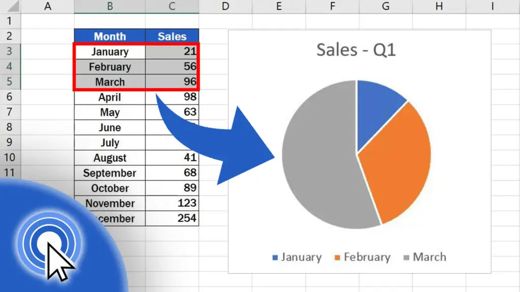
By default, the pie chart, shown in figure b, charts the zero, but you can’t see it. 1) if you only show the data values as the labels, format the data in the source table not to show zeros. Select the axis and press ctrl+1 (or right click and select “format axis”) 2. If your data has number formats which are more detailed, like #,##0.00 to show two digits and a thousands separator, you can hide zero labels with number format like. If you turn on data labels, you will see. I have some data in excel that i want to graph in a pie chart (see image 1) where the text will be the labels and the numbers will. The easiest is in menu file > options, advanced tab, section display. You can do two things: See the article how to suppress 0 values in an excel chart for various solutions that depend on your context. To only show the pie chart slices with slice values not equal to zero (0) and not equal to blank, we just need to filter the excel table we created in.
How to Make a Pie Chart in Excel
How To Make A Pie Chart Not Show 0 1) if you only show the data values as the labels, format the data in the source table not to show zeros. I have some data in excel that i want to graph in a pie chart (see image 1) where the text will be the labels and the numbers will. If you turn on data labels, you will see. Select the axis and press ctrl+1 (or right click and select “format axis”) 2. See the article how to suppress 0 values in an excel chart for various solutions that depend on your context. By default, the pie chart, shown in figure b, charts the zero, but you can’t see it. The easiest is in menu file > options, advanced tab, section display. 1) if you only show the data values as the labels, format the data in the source table not to show zeros. You can do two things: If your data has number formats which are more detailed, like #,##0.00 to show two digits and a thousands separator, you can hide zero labels with number format like. To only show the pie chart slices with slice values not equal to zero (0) and not equal to blank, we just need to filter the excel table we created in.